Detector model interface
In addition to the neutrino data itself, the IceCube collaboration provides some information about the detector that can be useful to construct simple simulations and fits. For example, the effective area is needed to connect between incident neutrino fluxes and expected number of events in the detector.
icecube_tools also provides an quick interface to loading and working with such information. This is a work in progress and only certain datasets are currently implemented, such as the ones demonstrated below.
[1]:
import numpy as np
from matplotlib import pyplot as plt
from matplotlib.colors import LogNorm

from icecube_tools.utils.data import IceCubeData
from icecube_tools.detector.detector import IceCube, TimeDependentIceCube
The IceCubeData class can be used for a quick check of the available datasets on the IceCube website.
[2]:
my_data = IceCubeData()
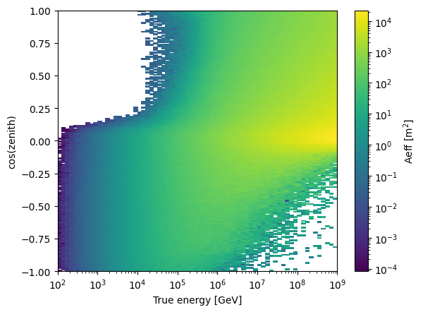
Effective area, angular resolution and energy resolution of 10 year data
We can now use the date string to identify certain datasets. Let’s say we want to use the effective area and angular resolution from the 20210126 dataset. If you don’t already have the dataset downloaded, icecube_tools will do this for you automatically. This 10 year data release provides more detailed IRF data.
We restrict our examples to the Northern hemisphere.
The simpler, earlier versions are explained afterwards.
The format of the effective area has not changed, though.
For this latest data set, we have different detector configurations available, as they changed through time (the detector was expanded). We can invoke a chosen configuration throught the second argument in EffectiveArea.from_dataset() for this particular data set only.
[3]:
from icecube_tools.detector.r2021 import R2021IRF
from icecube_tools.detector.effective_area import EffectiveArea
[4]:
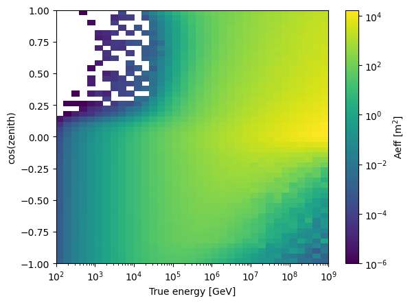
my_aeff = EffectiveArea.from_dataset("20210126", "IC86_II")
20210126: 39843820it [00:18, 2151653.52it/s]
[5]:
fig, ax = plt.subplots()
h = ax.pcolor(
    my_aeff.true_energy_bins, my_aeff.cos_zenith_bins, my_aeff.values.T, norm=LogNorm()
)
cbar = fig.colorbar(h)
ax.set_xscale("log")
ax.set_xlim(1e2, 1e9)
ax.set_xlabel("True energy [GeV]")
ax.set_ylabel("cos(zenith)")
cbar.set_label("Aeff [m$^2$]")
Energy resolution
Angular resolution depends on the energy resolution. The paper accompaying the data release explains the dependency: For each bin of true energy and declination a certain amount of events is simulated. These are sorted first into bins of reconstructed energy. These are then reconstructed in terms of PSF(the kinematic angle between the incoming neutrino and the outgoing muon after a collision) and actual angular error. Data is given as fractional
counts in the bin \((E_\mathrm{reco}, \mathrm{PSF}, \mathrm{ang\_err})\) of all counts in bin (E_:nbsphinx-math:mathrm{true}, \delta). This is nothing but a histogram, corresponding to a probability of finding an event with given true energy and true declination: \(p(E_\mathrm{reco}, \mathrm{PSF}, \mathrm{ang\_err} \vert E_\mathrm{true}, \delta)\).
We find the energy resolution, i.e. \(p(E_\mathrm{reco} \vert E_\mathrm{true}, \delta)\), by summing over (marginalising over) all entries of \(\mathrm{PSF}, \mathrm{ang\_err}\) for the reconstructed energy we are interested in.
The R2021IRF()class is able to do so:
[6]:
irf = R2021IRF.from_period("IC86_II")
[7]:
fig, ax = plt.subplots()
idx = [0, 3, 6, 9, 12]
# plotting Ereco for different true energy bins, the declination bin here is always from +10 to +90 degrees.
for i in idx:

    x = np.linspace(*irf.reco_energy[i, 2].support(), num=1000)
    ax.plot(x, irf.reco_energy[i, 2].pdf(x), label=irf.true_energy_bins[i])
ax.legend()
[7]:
<matplotlib.legend.Legend at 0x7f16fd9738e0>
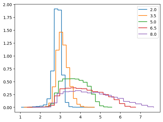
This should look like the Fig.4, left panel, of the mentioned paper, the y-axis is only scaled by a constant factor, corresponding to a properly normalised distribution. On this topic, it should be mentioned that the quantities distributed according to these histograms are the logarithms of reconstructed energy, PSF and angular uncertainty! Accordingly, logarithmic quantities are drawn as samples and only exponentiated for calculations and final data products.
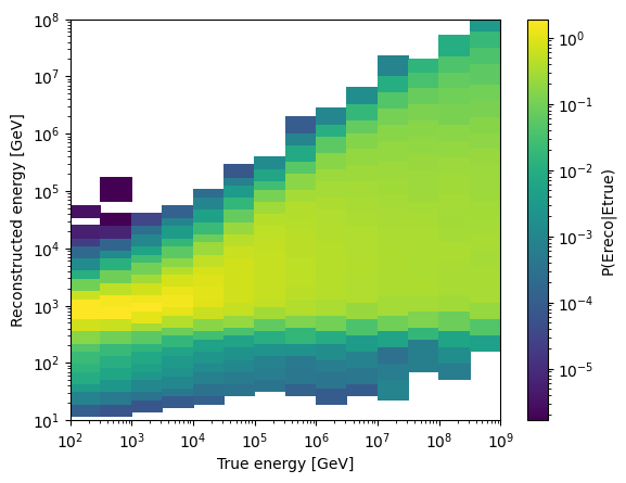
Etrue vs. Ereco
Below, a colormap of the conditional probability \(P(E_\mathrm{reco} \vert E_\mathrm{true})\) is shown. It is normalised for each Etrue bin.
[8]:
etrue = irf.true_energy_bins
ereco = np.linspace(1, 8, num=100)
[9]:
vals = np.zeros((etrue.size - 1, ereco.size - 1))
for c, et in enumerate(etrue[:-1]):
    vals[c, :] = irf.reco_energy[c, 2].pdf(ereco[:-1])
[10]:
fig, ax = plt.subplots()
h = ax.pcolor(np.power(10, etrue), np.power(10, ereco), vals.T, norm=LogNorm())
cbar = fig.colorbar(h)
ax.set_xlim(1e2, 1e9)
ax.set_ylim(1e1, 1e8)
ax.set_xscale("log")
ax.set_yscale("log")
ax.set_xlabel("True energy [GeV]")
ax.set_ylabel("Reconstructed energy [GeV]")
cbar.set_label("P(Ereco|Etrue)")
Angular resolution
Now that we have the reconstructed energy for an event with some \(E_\mathrm{true}, \delta\), we can proceed in finding the angular resolution.
First, from the given “history” of the event, we sample the matching distribution/histogram of \(\mathrm{PSF}\), again by marginalising over the uninteresting quantities, in this case only \(\mathrm{ang\_err}\). We thus sample a value of \(\mathrm{PSF}\), to whom a distribution of \(\mathrm{ang\_err}\) belongs, which we subsequently sample. This is now to be understood as a cone of a given angular radius, within which the true arrival direction lies with a probability of 50%.
For both steps, the histograms are created by R2021IRF() when instructed to do so: we pass a tuple of vectors (ra, dec) in radians and a vector of \(\log_{10}(E_\mathrm{true})\) to the method sample(). Returned are sampled ra, dec (both in radians), angular error (68%, in degrees) and reconstructed energy in GeV.
[11]:
irf.sample((np.full(4, np.pi), np.full(4, np.pi / 4)), np.full(4, 2))
[11]:
(array([3.14460667, 3.1122957 , 3.1715669 , 3.12988768]),
 array([0.795381  , 0.80942401, 0.78207633, 0.7897252 ]),
 array([0.81314284, 1.18484801, 0.8403489 , 1.56147217]),
 array([ 638.4537496 , 1580.39481862,  985.08856794,  837.29002682]))
If you are interested in the actual distributions, they are accessible through the attributes R2021IRF().reco_energy (2d numpy array storing scipy.stats.rv_histogram instances) and R2021IRF().maginal_pdf_psf (a modified ditionary class instance, indexed by a chain of keys):
[12]:
etrue_bin = 0
dec_bin = 2
ereco_bin = 10
print(irf.marginal_pdf_psf(etrue_bin, dec_bin, ereco_bin, "bins"))
print(irf.marginal_pdf_psf(etrue_bin, dec_bin, ereco_bin, "pdf"))
[-3.13065092 -2.86582289 -2.60084567 -2.33592241 -2.07109231 -1.80631897
 -1.54136215 -1.27646224 -1.01153023 -0.74666199 -0.48174935 -0.21688286
  0.04805317  0.31281183  0.57772152  0.84267163  1.10754913  1.37235958
  1.63728955  1.90222053  2.1670218 ]
<scipy.stats._continuous_distns.rv_histogram object at 0x7f16fda70760>
The same works for marginal_pdf_angerr. The entries are only created once the sample() method needs to. See the class defintion of ddict in icecube_tools.utils.data for more details.
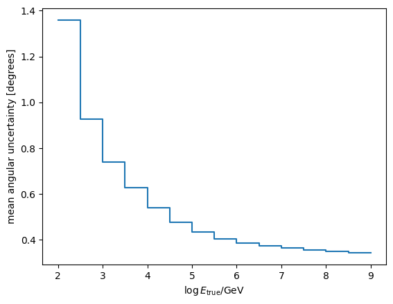
Mean angular uncertainty
We can find the mean angular uncertainty by sampling a large amount of events for different true energies, assuming that the average is sensibly defined as the average of logarithmic quantities.
[13]:
num = 10000
loge = irf.true_energy_bins
mean_uncertainty = np.zeros(loge.shape)
for c, e in enumerate(loge[:-1]):
    _, _, samples, _ = irf.sample(
        (np.full(num, np.pi), np.full(num, np.pi / 4)), np.full(num, e)
    )
    mean_uncertainty[c] = np.power(10, np.average(np.log10(samples)))
mean_uncertainty[-1] = mean_uncertainty[-2]
plt.step(loge, mean_uncertainty, where="post")
plt.xlabel("$\log E_\mathrm{true} / \mathrm{GeV}$")
plt.ylabel("mean angular uncertainty [degrees]")
[13]:
Text(0, 0.5, 'mean angular uncertainty [degrees]')
Constructing a detector
A detector used for e.g. simulations can be constructed from angular/energy uncertainties and an effective area:
[14]:
detector = IceCube(my_aeff, irf, irf, "IC86_II")
irf = R2021IRF() is used both as spatial and energy resolution, because it encompasses both types of information and inherits from both classes.
Time dependent detector
We can construct a “meta-detector” spanning multiple data periods through the class TimeDependentIceCube from strings defining the data periods. Alternatively, a
[15]:
tic = TimeDependentIceCube.from_periods("IC86_I", "IC86_II")
tic.detectors
/opt/hostedtoolcache/Python/3.9.20/x64/lib/python3.9/site-packages/icecube_tools/detector/r2021.py:89: RuntimeWarning: divide by zero encountered in log10
  self.dataset[:, 6:-1] = np.log10(self.dataset[:, 6:-1])
Empty true energy bins at: [(0, 0), (1, 0)]
[15]:
{'IC86_I': <icecube_tools.detector.detector.IceCube at 0x7f16fd942670>,
 'IC86_II': <icecube_tools.detector.detector.IceCube at 0x7f16fc450dc0>}
Available periods are
[16]:
TimeDependentIceCube._available_periods
[16]:
['IC40', 'IC59', 'IC79', 'IC86_I', 'IC86_II']
Effective area, angular resolution and energy resolution of earlier releases
Repeating the prodecure for the 20181018 dataset.
[17]:
from icecube_tools.detector.effective_area import EffectiveArea
from icecube_tools.detector.energy_resolution import EnergyResolution
from icecube_tools.detector.angular_resolution import AngularResolution
[18]:
my_aeff = EffectiveArea.from_dataset("20181018")
my_angres = AngularResolution.from_dataset("20181018")
/opt/hostedtoolcache/Python/3.9.20/x64/lib/python3.9/site-packages/icecube_tools/detector/effective_area.py:379: FutureWarning: The 'delim_whitespace' keyword in pd.read_csv is deprecated and will be removed in a future version. Use ``sep='\s+'`` instead
  output = pd.read_csv(
/opt/hostedtoolcache/Python/3.9.20/x64/lib/python3.9/site-packages/icecube_tools/detector/angular_resolution.py:111: FutureWarning: The 'delim_whitespace' keyword in pd.read_csv is deprecated and will be removed in a future version. Use ``sep='\s+'`` instead
  output = pd.read_csv(
[19]:
fig, ax = plt.subplots()
h = ax.pcolor(
    my_aeff.true_energy_bins, my_aeff.cos_zenith_bins, my_aeff.values.T, norm=LogNorm()
)
cbar = fig.colorbar(h)
ax.set_xscale("log")
ax.set_xlabel("True energy [GeV]")
ax.set_ylabel("cos(zenith)")
cbar.set_label("Aeff [m$^2$]")
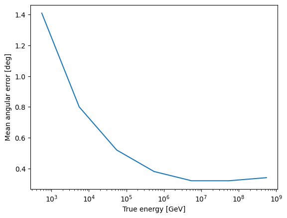
[20]:
fig, ax = plt.subplots()
ax.plot(my_angres.true_energy_values, my_angres.values)
ax.set_xscale("log")
ax.set_xlabel("True energy [GeV]")
ax.set_ylabel("Mean angular error [deg]")
[20]:
Text(0, 0.5, 'Mean angular error [deg]')
We can also easily check what datasets are supported by the different detector information classes:
[21]:
EffectiveArea.supported_datasets
[21]:
['20131121', '20150820', '20181018', '20210126']
[22]:
AngularResolution.supported_datasets
[22]:
['20181018']
[23]:
EnergyResolution.supported_datasets
[23]:
['20150820']
If you would like to see some other datasets supported, please feel free to open an issue or contribute your own!
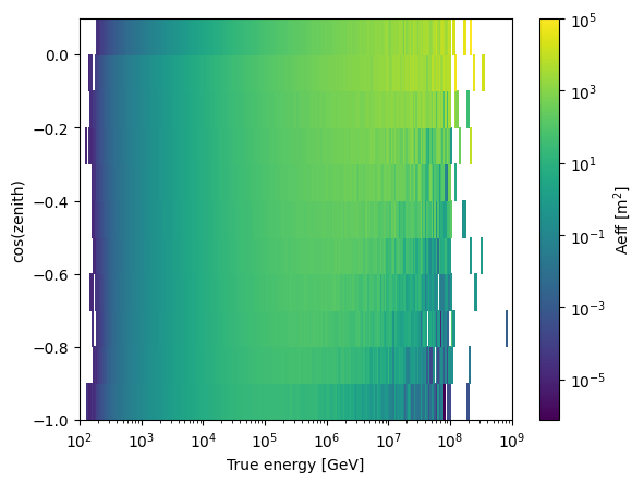
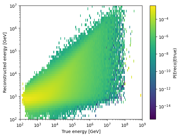
For the 20150820 dataset, for which we also have the energy resolution available…
[24]:
my_aeff = EffectiveArea.from_dataset("20150820")
my_eres = EnergyResolution.from_dataset("20150820")
20150820: 43711022it [00:00, 79686826.45it/s]
[25]:
fig, ax = plt.subplots()
h = ax.pcolor(
    my_aeff.true_energy_bins, my_aeff.cos_zenith_bins, my_aeff.values.T, norm=LogNorm()
)
cbar = fig.colorbar(h)
ax.set_xscale("log")
ax.set_xlabel("True energy [GeV]")
ax.set_ylabel("cos(zenith)")
cbar.set_label("Aeff [m$^2$]")
[26]:
fig, ax = plt.subplots()
h = ax.pcolor(
    my_eres.true_energy_bins, my_eres.reco_energy_bins, my_eres.values.T, norm=LogNorm()
)
cbar = fig.colorbar(h)
ax.set_xscale("log")
ax.set_yscale("log")
ax.set_xlabel("True energy [GeV]")
ax.set_ylabel("Reconstructed energy [GeV]")
cbar.set_label("P(Ereco|Etrue)")
Detector model
We can bring together these properties to make a detector model that can be used for simulations.
[27]:
from icecube_tools.detector.detector import IceCube
[28]:
my_detector = IceCube(my_aeff, my_eres, my_angres)
[ ]: