3. Model checking

Last time we focussed on building a simple initial model for the Cepheid variable data. In this notebook, we explore the next steps in the workflow, model implementation and model checking. Along the way, we’ll also introduce prior predictive checks and posterior predictive checks.

Implementation in Stan

In the model building notebook, we developed a simple model to fit the period-luminosity relation of Cepheid variable stars. We can now implement this model in Stan and use it to infer the parameters \(\alpha\) and \(\beta\) that describe the relation.

As we’ve seen before in the introduction notebook, Stan files consist of different blocks that divide information into data, parameters and model. You can find more detailed information on how to write models in Stan code here, but for now we can just take a look at this model: stan/cepheid_v0.stan.

!cat stan/cepheid_v0.stan

/**
 * Initial model for Cepheid variables
 * - Single galaxy
 * - Shared sigma_m
 **/

data {

  /* usual inputs */
  int Nc; // number of Cepheids
  vector[Nc] m_obs; // obs apparent mag.
  real sigma_m; // mag uncertainty
  vector[Nc] log10P; // log10(periods/days)
  real z; // redshift of single galaxy

  /* for generated quantities */
  int Ngrid;
  vector[Ngrid] log10P_grid;
}

transformed data {

  real dL;

  /* luminosity distance */
  dL = (3.0e5 * z) / 70.0; // Mpc

}

parameters {

  /* parameters of the P-L relation */
  real alpha;
  real beta;

}

transformed parameters {

  vector[Nc] M_true;
  vector[Nc] m_true;

  /* P-L relation */
  M_true = alpha + beta * log10P;

  /* convert to m */
  m_true = M_true + 5 * log10(dL) + 25;

}

model {

  /* likelihood */
  m_obs ~ normal(m_true, sigma_m);

}

generated quantities {

  vector[Ngrid] line;

  /* generate the posterior for the P-L relation */
  line = alpha + beta * log10P_grid;

}

A few things to note:

• We could have left the M <-> m conversion outside of Stan for a more compact program, but it is quite easy to have it inside, meaning that our work in this notebook is simplified.

• We could cut out the transformed parameters block and replace m_true with a long expression in the model block, but this is easy to read and gives us direct access to the M_true and m_true distributions, as we will see later.

• The generated quantities block is not part of the statistical model, but is run once for every iteration of the sampler. This can be useful for generating simple outputs, again as we will see later.

What about priors??

The more awake amongst you may notice that we have explicitly specified data, parameters and a likelihood in the Stan code, but no prior. A Bayesian analysis requires specification of the priors, so what is going on? By default, Stan will assume a uniform prior over the range of the parameters that you specified. Here, we specify alpha and beta with no bounds, and so our prior is implicitly uniform over all the real numbers. Does this sound reasonable? In any case, we will run with it for now, and talk about priors more later in this notebook.

Next, let’s set up our environment and compile our model to get ready to fit some data.

import numpy as np
from matplotlib import pyplot as plt
import arviz as av
from cmdstanpy import CmdStanModel

cepheid_v0 = CmdStanModel(stan_file="stan/cepheid_v0.stan")

INFO:cmdstanpy:found newer exe file, not recompiling
INFO:cmdstanpy:compiled model file: /Users/fran/projects/BayesianWorkflow/src/notebooks/stan/cepheid_v0

The first check: fitting simulated data

While we developed our initial generative and statistical models with the goal to fit real data, in doing so we now have a simple simulation program that contains exactly the same information as is included in our model. We can use this to generate simulated data where we know the values of alpha and beta, and can verify that our fit gives us reasonable results.

If we are not able to recover the known simulated truth, this means there is some kind of discrepancy between the generative model and the statistical model. This fact can be a powerful tool for debugging, especially when working with more complex models, as it allows us to check if our Stan model is doing what we think it should be. Just because it compiles, it doesn’t mean that it is correct!

So, let’s use our work in the model building to simulate a test dataset using the same assumptions that we did there:

# known quantities
z = 0.005

Nc = 10
P = [71.5, 45.0, 19.9, 30.6, 8.8, 75.2, 21.5, 22.0, 34.5, 87.4] # days
sigma_m = 0.5

c = 3.0e5 # km/s
H0 = 70.0 # km/s/Mpc

# high-level parameter values
alpha_true = -2
beta_true = -4

You can copy over your simulation code, or load data that you saved last time. I’ll load some data that I simulated earlier:

m_obs = np.array([21.30057715, 22.89477067, 24.63106411,
                  22.72569458, 26.29936958, 22.34729756,
                  24.19867534, 24.64700615, 23.19478031, 21.94968928])

We can now define our data dict to pass to the Stan model…

Note: The variable names in the Stan file must match the keys of the dict

data = {}
data["Nc"] = Nc
data["z"] = z
data["log10P"] = np.log10(P)
data["m_obs"] = m_obs
data["sigma_m"] = sigma_m

# for generated quantities
data["Ngrid"] = 50
data["log10P_grid"] = np.linspace(0, 3)

… and try to fit the simulated data

# run fit
fit = cepheid_v0.sample(data=data, iter_sampling=1000, chains=4)

# check diagnostics
fit.diagnose();

# print summary
fit.summary()

INFO:cmdstanpy:start chain 1
INFO:cmdstanpy:start chain 2
INFO:cmdstanpy:start chain 3
INFO:cmdstanpy:start chain 4
INFO:cmdstanpy:finish chain 2
INFO:cmdstanpy:finish chain 1
INFO:cmdstanpy:finish chain 3
INFO:cmdstanpy:finish chain 4
INFO:cmdstanpy:Processing csv files: /var/folders/8d/cyg0_lx54mggm8v350vlx91r0000gn/T/tmpmlkdxck8/cepheid_v0-202108271019-1-hce0fjz2.csv, /var/folders/8d/cyg0_lx54mggm8v350vlx91r0000gn/T/tmpmlkdxck8/cepheid_v0-202108271019-2-ecyi9p7i.csv, /var/folders/8d/cyg0_lx54mggm8v350vlx91r0000gn/T/tmpmlkdxck8/cepheid_v0-202108271019-3-_xo9pdvk.csv, /var/folders/8d/cyg0_lx54mggm8v350vlx91r0000gn/T/tmpmlkdxck8/cepheid_v0-202108271019-4-j47jnkvj.csv

Checking sampler transitions treedepth.
Treedepth satisfactory for all transitions.

Checking sampler transitions for divergences.
No divergent transitions found.

Checking E-BFMI - sampler transitions HMC potential energy.
E-BFMI satisfactory.

Effective sample size satisfactory.

Split R-hat values satisfactory all parameters.

Processing complete, no problems detected.

	Mean	MCSE	StdDev	5%	50%	95%	N_Eff	N_Eff/s	R_hat
name
lp__	-4.8	0.0320	1.00	-6.9	-4.5	-3.800	1000.0	4300.0	1.0
alpha	-1.3	0.0340	0.83	-2.7	-1.3	0.036	590.0	2500.0	1.0
beta	-4.5	0.0220	0.54	-5.4	-4.5	-3.600	580.0	2500.0	1.0
M_true[1]	-9.7	0.0076	0.24	-10.0	-9.7	-9.300	1016.0	4304.0	1.0
M_true[2]	-8.8	0.0036	0.18	-9.1	-8.8	-8.500	2440.0	10341.0	1.0
...	...	...	...	...	...	...	...	...	...
line[46]	-14.0	0.0270	0.68	-15.0	-14.0	-13.000	621.0	2633.0	1.0
line[47]	-14.0	0.0290	0.72	-15.0	-14.0	-13.000	618.0	2620.0	1.0
line[48]	-14.0	0.0300	0.75	-16.0	-14.0	-13.000	614.0	2603.0	1.0
line[49]	-15.0	0.0320	0.78	-16.0	-15.0	-13.000	612.0	2592.0	1.0
line[50]	-15.0	0.0330	0.81	-16.0	-15.0	-14.000	609.0	2582.0	1.0

73 rows × 9 columns

# to access chains of parameter values
alpha_chain = fit.stan_variable("alpha")

# plot trace
av.plot_trace(fit, var_names=["alpha", "beta", "m_true"]);

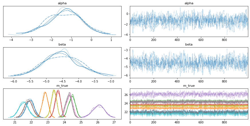
So by including m_true in the transformed parameters block, we also get the marginal distributions ready-made for free. Different chains have different linestyles and different Cepheids have different colours in this plot.

Exercise 1 (5 points): Looking closely, it seems that the m_true distributions vary from star to star, with medium m_true values having narrower distributions. We know sigma_m is fixed, so why might this be?

ax = av.plot_pair(fit, var_names=["alpha", "beta"], marginals=True)

# overlay truth in red
ax[1,0].axvline(alpha_true, color="r")
ax[1,0].axhline(beta_true, color="r")

<matplotlib.lines.Line2D at 0x1467e8d60>

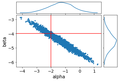
We can see that we are able to recover the true result, although alpha and beta are quite correlated. Going back to the fit summary, we see that the number of effective samples is quite low - only ~500 for 4x1000 iterations! This fit is very fast and so we could just run it longer, but a common reparametrisation for slopes and intercepts could make the sampling much more efficient.

Exercise 2 (5 points): Try using the following reparametrisation for the period-luminosity relation:

\[y = \alpha + \beta x \rightarrow y = \alpha^\prime + \beta (x - x_0)\]

where \(x_0\) is the mean value of \(x\), typically called the pivot. Compare the number of effective samples with the previous version. Additionally, compare the joint posterior for alpha and beta with that for alpha_prime and beta. Why is this parametrisation so much more efficient?

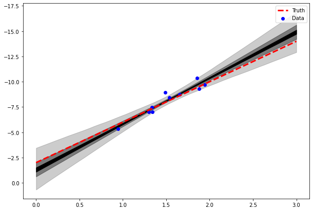
We can also use our generated quantities block to quickly visualise the posterior for the line fit:

line = fit.stan_variable("line")

# 4x1000 iterations, grid of Ngrid points
np.shape(line)

(4000, 50)

# get M_obs
dL = (c * z) / H0
M_obs = m_obs - 25 - 5 * np.log10(dL)

# for plot
Np = 200
log10P_grid = data["log10P_grid"]
line = fit.stan_variable("line")

fig, ax = plt.subplots()
fig.set_size_inches(10, 7)

# approximate X% regions of highest posterior density
level = 99 #%
ax.fill_between(log10P_grid, np.percentile(line, 50 - 0.5*level, axis=0),
               np.percentile(line, 50 + 0.5*level, axis=0), color="k", alpha=0.2)
level = 60 #%
ax.fill_between(log10P_grid, np.percentile(line, 50 - 0.5*level, axis=0),
               np.percentile(line, 50 + 0.5*level, axis=0), color="k", alpha=0.4)
level = 20 #%
ax.fill_between(log10P_grid, np.percentile(line, 50 - 0.5*level, axis=0),
               np.percentile(line, 50 + 0.5*level, axis=0), color="k", alpha=1)
ax.scatter(np.log10(P), M_obs, color="b", label="Data")
ax.plot(log10P_grid, alpha_true + beta_true * log10P_grid, color="r", lw=3,
        linestyle="--", label="Truth")
ax.invert_yaxis()
ax.legend()

<matplotlib.legend.Legend at 0x1466eadf0>

Prior selection and prior predictive checks

As discussed in Section 3.1, we left our priors for alpha and beta to be uniform over all real numbers. In the end, this didn’t seem to be a major problem and the data were informative enough to constrain the posterior. However, we should be wary of these kind of uninformative priors. The first motivation is common sense - from studying the data and literature, we have a fairly good idea of what the period-luminosity relationship looks like. Additionally, our sampler currently has to consider alpha and beta values from negative to positive infinity.

It is rarely the case that we have zero prior knowledge on the value of our model parameters. At the same time, we don’t want to bias our results by introduing too much information with so-called informative priors. After all, we are trying to find out what the values of alpha and beta are.

Like many things in life, there is a happy medium between these two extremes that we can use in practice. Weakly informative priors are wide enough to reflect our ignorance, but narrow enough to constrain the parameter space to sensible values. The exact shape of a weakly informative prior should have negligible impact on the fit results.

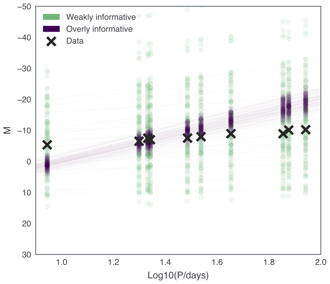
To help us choose sensible informative priors, we can use prior predictive checks. This just means sampling from the prior distribution in your generative model, and comparing the resulting data with your actual data. The idea is that the prior predictive data should cover a wide enough region to cover all reasonable data values, and visualising priors this way in the “data-space” can be helpful in prior selection.

Exercise 3 (5 points): Expand your generative model to sample from the prior distributions for alpha and beta. Plot the resulting data (m_obs and P) for a few different choices of prior distributions.

# to be completed
#alpha = np.random...
#beta = np.random...

# simulation as before

# plot for different assumptions

Your results should look something like the following:

For our problem, let’s update the Stan model with the following priors:

\[\alpha \sim N(0, 10)\]

\[\beta \sim N(-5, 5)~\rm{for}~\beta \lt 0,\]

where the extra constraint on \(\beta\) reflects the fact that we expect a negative slope.

The new stan model can be found in stan/cepheid_v1.stan. Note the <upper=0> syntax for parameter bounds and the new priors in the model block.

!cat stan/cepheid_v1.stan

/**
 * Initial model for Cepheid variables
 * - Single galaxy
 * - Shared sigma_m
 * - Weakly informative priors
 **/

data {

  /* usual inputs */
  int Nc; // number of Cepheids
  vector[Nc] m_obs; // obs apparent mag.
  real sigma_m; // mag uncertainty
  vector[Nc] log10P; // log10(periods/days)
  real z; // redshift of single galaxy

  /* for generated quantities */
  int Ngrid;
  vector[Ngrid] log10P_grid;
}

transformed data {

  real dL;

  /* luminosity distance */
  dL = (3.0e5 * z) / 70.0; // Mpc

}

parameters {

  /* parameters of the P-L relation */
  real alpha;
  real<upper=0> beta;

}

transformed parameters {

  vector[Nc] M_true;
  vector[Nc] m_true;

  /* P-L relation */
  M_true = alpha + beta * log10P;

  /* convert to m */
  m_true = M_true + 5 * log10(dL) + 25;

}

model {

  /* priors */
  alpha ~ normal(0, 10);
  beta ~ normal(-5, 5);

  /* likelihood */
  m_obs ~ normal(m_true, sigma_m);

}

generated quantities {

  vector[Ngrid] line;

  /* generate the posterior for the P-L relation */
  line = alpha + beta * log10P_grid;

}

Let’s fit this model instead, and see how it performs.

stan_model = CmdStanModel(stan_file="stan/cepheid_v1.stan")
fit = stan_model.sample(data=data, iter_sampling=1000, chains=4)

INFO:cmdstanpy:found newer exe file, not recompiling
INFO:cmdstanpy:compiled model file: /Users/fran/projects/BayesianWorkflow/src/notebooks/stan/cepheid_v1
INFO:cmdstanpy:start chain 1
INFO:cmdstanpy:start chain 2
INFO:cmdstanpy:start chain 3
INFO:cmdstanpy:start chain 4
INFO:cmdstanpy:finish chain 1
INFO:cmdstanpy:finish chain 2
INFO:cmdstanpy:finish chain 3
INFO:cmdstanpy:finish chain 4

# for plot
log10P_grid = data["log10P_grid"]
line = fit.stan_variable("line")

fig, ax = plt.subplots()
fig.set_size_inches(10, 7)

# approximate X% regions of highest posterior density
level = 99 #%
ax.fill_between(log10P_grid, np.percentile(line, 50 - 0.5*level, axis=0),
               np.percentile(line, 50 + 0.5*level, axis=0), color="k", alpha=0.2)
level = 60 #%
ax.fill_between(log10P_grid, np.percentile(line, 50 - 0.5*level, axis=0),
               np.percentile(line, 50 + 0.5*level, axis=0), color="k", alpha=0.4)
level = 20 #%
ax.fill_between(log10P_grid, np.percentile(line, 50 - 0.5*level, axis=0),
               np.percentile(line, 50 + 0.5*level, axis=0), color="k", alpha=1)
ax.plot(log10P_grid, alpha_true + beta_true * log10P_grid, color="r", lw=3,
        linestyle="--", label="Truth")
ax.invert_yaxis()
ax.legend()

<matplotlib.legend.Legend at 0x1463d2400>

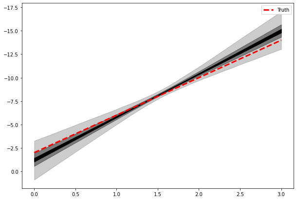
We see that the prior choice has negligible impact on the results.

Exercise 4 (5 points): Experiment with stronger priors and/or weaker data to see how this affects the inferred relation. Make some plots to visualise your results.

# to be completed...

Posterior predictive checks

If our model fits the data well, then data generated by the model should look similar to observed data. To test if this is true, we can perform a posterior predictive check.

If we have observed data \(\hat{m}\) and model parameters \(\alpha\) and \(\beta\), we can express the joint posterior predictive distribution as

\[p(\hat{m}_\mathrm{rep} | \hat{m}) = \int \mathrm{d}\alpha \int \mathrm{d}\beta~p(\hat{m}_\mathrm{rep}| \alpha, \beta) p(\alpha, \beta | \hat{m}),\]

where \(\hat{m}_\mathrm{rep}\) is the replicated data predicted by our fitted model. We can think of this as the data our model predicts we should see in future.

In practice, we can easily compute this integral using the Markov chains that we get from Stan. All we have to do is use the posterior samples for \(\alpha\) and \(\beta\) to forward simulate data from our likelihood, or generative model.

Exercise 5 (5 points): Let’s compute the posterior predictive distribution for our fit to simulated data…

alpha_chain = fit.stan_variable("alpha")
beta_chain = fit.stan_variable("beta")

Nreps = 250

# to be completed...
# sample Nreps alpha and beta from chains
# for each, simulate to get m_obs_rep
# plot comparison of many simulated m_obs_rep datasets with m_obs used in fit
# or equivalently for M_obs_rep/M_obs

Your results should look something like the following:

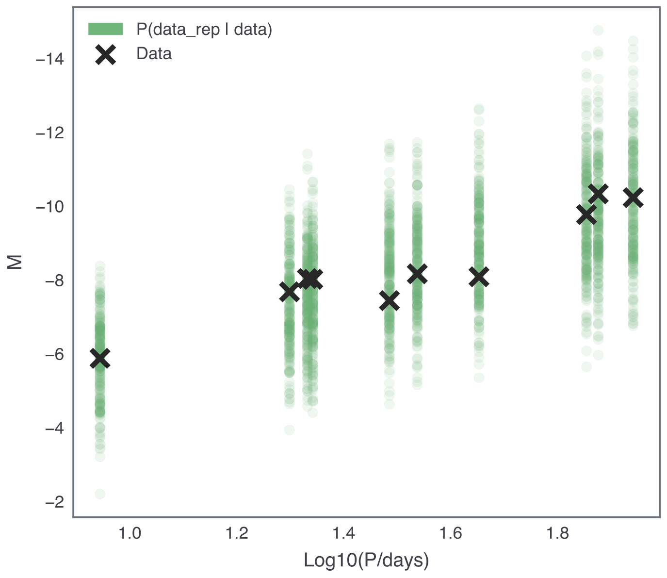
There are a number of ways to study and quantify the posterior predictive distribution in order to use it to assess the “goodness of fit” of a model. Here, we only consider graphical checks, but more information can be found in Section 6.3 of Bayesian Data Analysis by Gelman et al.

Application to actual data

Homework exercise 1 (20 points): Now, let’s use our cepheid_v1.stan model to fit the actual data introduced in the model building notebook. Here we have a model for one galaxy only, so let’s pick one at random to start with. Complete the following steps:

• Note that the actual data have individual sigma_m for each Cepheid. We want to use as much information as possible, so quickly expand the Stan model to include this.

• Load the data into Stan and perform a fit. Make a plot summarising the posterior of the line fit and compare it to the M_obs data values.

• Complete a posterior predictive check for this fit.

• Repeat steps 2 and 3 for a few other galaxies to compare. Comment on the overall results.

# to be completed...

The above exercise should leave us feeling unsatisfied with out model. We seek out an expert to discuss with, and learn the following information: * The metallicity of a Cepheid has a systematic effect on its intrinsic brightness, shifting it by a factor of \(\gamma=1.5\) * We don’t know the uncertainty in the observed period values - it is likely small, but maybe it is not measured perfectly. * The frequency or “cadence” of astronomical observations means that it is only possible to measure certain periods.

Homework exercise 2 (30 points): Use the above information together with the completed posterior predictive checks to improve your Stan model. Some changes may be more useful than others, so it can be good to test each in isolation. Once you are satisfied with your single galaxy model, save it as cepheid_v2.stan, and make some plots arguing your case.

# to be completed...

Homework exercise 3 (30 points): Use your improved model, cepheid_v2.stan to fit the data from each galaxy independently. Make some plots showing the resulting alpha and beta marginal posteriors for the different galaxies (e.g. ridgeline plots can be a nice way to show this). What can you conclude about the universailty of the period-luminosity relation?

# to be completed...

Further reading

• Weakly informative priors: Simpson, D., Rue, H., Riebler, A., Martins, T. G. & Sørbye, S. H. Penalising Model Component Complexity: A Principled, Practical Approach to Constructing Priors. Statistical Science 32, 1–28 (2017). DOI: 10.1214/16-STS576.

• Posterior predictive checks: Section 6.3 of Bayesian Data Analysis by Gelman et al.